GPTQ, with the code open

Method

What quantization is, and why anyone bothers

Start with the physical problem. OPT-175B, the model the paper targets, has 175 billion weights. Each is stored as a 16-bit floating-point number (2 bytes), so the model occupies about 350 GB. That is too big for any single GPU, and size is not even the worst of it. To generate one token, the GPU must read essentially every weight from memory once. An A100 can read about 2 TB per second, so 350 GB of weights means roughly a sixth of a second per token spent on nothing but moving bytes. Weight size is generation speed.

Quantization attacks the bytes directly. Instead of letting each weight be any 16-bit number, you restrict it to a small menu of allowed values. With 4 bits per weight the menu has $2^4 = 16$ entries; with 3 bits, 8 entries. Each weight is then stored as a tiny integer saying which menu entry it uses, and the model shrinks four to five times. At 3 bits, OPT-175B fits on a single 80 GB A100, which is the paper’s headline demo.

What does the menu look like? GPTQ uses the simplest possible kind: sixteen evenly spaced tick marks, like a ruler, stretched to cover one row of weights. A concrete example from the code’s formulas: if a row’s weights span the range $[-0.8, +0.4]$, the step between ticks is

$$\text{scale} = \frac{0.4 - (-0.8)}{16 - 1} = 0.08 ,$$

and the sixteen allowed values are $-0.80, -0.72, -0.64, \dots, 0.00, \dots, +0.40$. Storing a weight means recording which tick it sits on (an integer from 0 to 15) plus, once per row, the ruler itself (the step size, and which tick represents zero; the code rounds that “zero point” to a whole tick so that the value 0.0 is always exactly representable, quant.py:76). Turning an integer back into a number is one multiply:

$$\hat w = \text{scale} \cdot (q - \text{zero}) .$$

The GPU kernel does this on the fly while multiplying, so the 4× fewer bytes translate almost directly into faster generation. Nothing about the menu is clever, and that’s a feature: all the intelligence goes into which tick each weight lands on.

The obvious approach, and how it fails

The obvious algorithm is: snap every weight to its nearest tick. This is called round-to-nearest, RTN in the tables below. Each individual error is at most half a step, which sounds harmless.

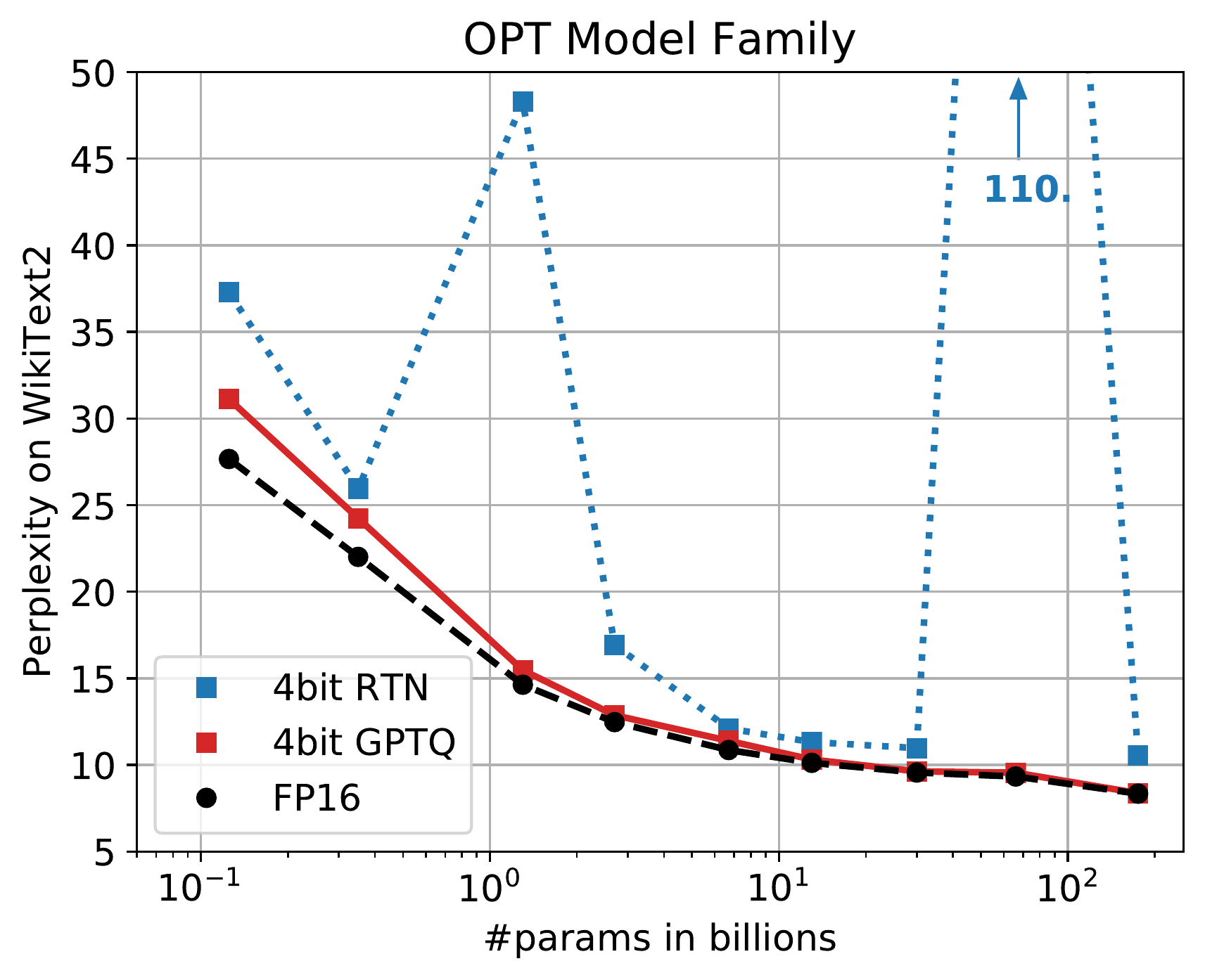
For OPT-175B at 4 bits, RTN raises the model’s error on test text by an order of magnitude. The model is ruined. And here is the part I find genuinely strange: the failure is not smooth in model size. Some OPT sizes tolerate RTN fine, then OPT-66B explodes, then 175B is bad again, and the sister model BLOOM survives RTN almost intact. You cannot test rounding on a small model and extrapolate. (The first figure under Benchmarks shows this jagged behavior; nobody fully understands which training choices make a model fragile this way.)

So the interesting question is not “are the individual errors small” but “what do thousands of small errors do together to the layer’s output”. That reframing is the entire method.

Measuring damage where it matters

A layer of the network computes, for each output, a weighted sum of its inputs: take the layer’s input numbers $x_1, x_2, \dots$, multiply each by a weight, add them up. The damage that matters is not “how far did each weight move” but “how much did that output sum change”, measured over real data.

One example makes the whole idea click. Suppose a neuron computes $y = w_1 x_1 + w_2 x_2$, with $w_1 = 0.63$ and $w_2 = -0.41$, and suppose that in real data $x_2$ always happens to equal $x_1$. Then

$$y = (0.63 - 0.41)\,x_1 = 0.22\,x_1 .$$

Only the sum of the two weights ever matters. If rounding forces $w_1$ down to $0.50$ (an error of $0.13$), I can add $0.13$ to $w_2$ and the neuron’s output is exactly what it was, on every input, forever. The individual weights are both “wrong” now; the behavior is untouched. I ran this as a numerical experiment with actual data: forcing the error alone changed the output error to 16.6 (in squared units); applying the fix brought it to $10^{-29}$, which is zero in floating point.

Real inputs are not perfectly correlated, but in a transformer they are heavily correlated, and partial correlation allows partial cancellation. To exploit this systematically you need two pieces of information about the calibration data (GPTQ uses 128 chunks of 2048 tokens from a web-text dataset):

• how “loud” each input is: inputs that are large and frequent make their weights expensive to round;
• how correlated each pair of inputs is: correlation is spare room for cancellation.

Both live in one matrix, $H = 2XX^\top$, where $X$ holds the calibration inputs. Its diagonal entries are the loudness of each input; its off-diagonal entries are the correlations. This matrix is called the Hessian, a general math term for “the matrix of second derivatives of some function”, but you don’t need that generality here: for the layer-output damage function, I verified numerically that $H = 2XX^\top$ is exactly the right damage-pricing matrix, not an approximation (finite-difference check, relative error $10^{-7}$). If you want the longer road, with what a Hessian is in general and why every row of the layer shares this one, I wrote a separate note on it.

The repair rule

Now the core question. Rounding just forced one weight, call it $w_q$, to move to its nearest tick, an error of $e = w_q - \mathrm{quant}(w_q)$ that we had no choice about. The weights not yet rounded (call that set $F$) are still free. Where should they move to cancel as much damage as possible?

Optimal Brain Surgeon (Hassibi & Stork, 1992) answers exactly this. The best adjustment is

$$\delta_F = -\,\frac{w_q - \mathrm{quant}(w_q)}{\left[H_F^{-1}\right]_{qq}}\ \cdot\ \left(H_F^{-1}\right)_{:,q} ,$$

which looks dense, so here is each piece in words. $H_F^{-1}$ is the inverse of the damage matrix, restricted to the still-free weights. Its column $(H_F^{-1})_{:,q}$ is a settling pattern: picture the weights as balls connected by springs whose stiffnesses are the entries of $H$; if you grab ball $q$ and yank it, this column is where every other ball comes to rest. The fraction out front scales that pattern so ball $q$ moves by exactly $-e$, its forced rounding error (you can substitute and check: the $q$-th component of $\delta_F$ collapses to $-e$). Everything else is the ripple.

For readers comfortable with constrained optimization: the formula is the exact solution of “minimize damage subject to $\delta_q = -e$” by Lagrange multipliers, three lines. For everyone else, here is the check that convinced me it’s right without trusting anyone’s algebra. I quantized one weight, applied the formula, and separately solved the same problem by brute force (exact least squares over the free weights). The two answers agree to fifteen decimal places.

And the two-input picture from before generalizes cleanly. If two inputs have correlation $\rho$ (a number between $-1$ and $1$; ours were $\rho = 1$), the formula works out to: the free weight absorbs a fraction $\rho$ of the error, and the damage shrinks to $(1-\rho^2)$ of what plain rounding leaves. At $\rho = 0.9$ that is a 5× reduction; at $\rho = 0$, no correlation, the formula does nothing and you’re back to RTN. I verified both predictions numerically across several values of $\rho$. One confession that belongs here: my first implementation of the formula had the sign of $e$ flipped, and the “repair” made everything worse. The brute-force baseline is what caught it. Sign errors in compensation code fail silently; build the dumb exact check first.

From one repair to a whole model

Turning the repair rule into an algorithm sounds easy: go through the weights one by one, snap each to its nearest tick, repair, repeat. The catch is cost. Each repair needs $H_F^{-1}$, the inverse for the currently free set, and every step shrinks that set, which genuinely changes the inverse (a sub-block of an inverse is not the inverse of the sub-block). The pre-GPTQ algorithm, OBQ, also greedily chose which weight to do next per row. Each of a layer’s thousands of rows then needs its own private sequence of thousands of recomputed inverses. For a 175B model, that adds up to years.

GPTQ’s contribution is noticing two enormous simplifications:

1. Give up choosing the order. Quantize columns plain left to right, the same order for every row. The paper’s ablation says the greedy choice was barely helping on large models. And once all rows share one order, they share the entire sequence of inverses; the linear algebra is paid once per layer instead of once per row.
2. Precompute the whole sequence at once. There is a standard factorization (Cholesky) with the property that, for a fixed left-to-right order, its rows contain every number the sequence of shrinking inverses will ever need. The code computes it in three lines (gptq.py:101–103), and the loop afterward just reads rows out of it. I checked the consistency of this against the repair formula: the loss the code tracks per weight, $(w-q)^2/(2d^2)$ at gptq.py:134, matches Optimal Brain Surgeon’s damage formula exactly when $d^2 = [H_F^{-1}]_{qq}$, which is the standard relation between a Cholesky factor and its sub-inverses. I did not re-derive that relation from scratch.

Plus one engineering trick: repairs within the current block of 128 columns happen immediately, and the repair to everything beyond the block is saved up and applied as one big matrix multiply (gptq.py:137 and 143), which is the shape of work GPUs like. Result: 175B quantized in about four hours on one GPU.

There is a subtle and, I think, beautiful interaction hiding in the loop. By the time a weight’s own turn comes, earlier repairs have already shifted it, so it gets snapped to the nearest tick of its shifted position, sometimes a different tick than its original value would have chosen. Each step is round-to-nearest, but the sequence as a whole makes coordinated rounding choices. A different paper, AdaRound, proved that per-weight nearest rounding is provably suboptimal precisely when inputs are correlated, and optimizes the round-up-or-down choices directly; GPTQ gets a greedy version of the same effect free, as a side effect of repair. The same drift has a sharp edge, though: the ruler for each row was fitted to the weights before any repairs ran (gptq.py:72–73), so a weight that drifts far enough can leave the ruler’s range entirely and get clamped to the end tick. Whether that clamping costs accuracy, nobody measures.

Paper vs. code

You don’t need to read code to use this section; it exists because the paper and the implementation are not quite the same object, and the differences are informative. Repo: IST-DASLab/gptq at commit 2d65066, the authors’ own. The entire algorithm is gptq.py, 171 lines.

What I could match directly:

Paper	Code
Damage matrix $H = 2XX^\top$	Built incrementally as a running mean over calibration batches, gptq.py:53–58. Same matrix up to a harmless constant factor.
Stabilize $H$ by adding 1% of its mean diagonal	gptq.py:98–100, default percdamp=.01 in opt.py:380
Cholesky reformulation	gptq.py:101–103
Batched repairs, block size 128	gptq.py:106 (loop) and 143 (deferred update)
128 calibration samples from C4	opt.py:376 (default), datautils.py:54

What the code does that the paper doesn’t tell you:

• Inputs that are completely silent across all 128 calibration samples make $H$ non-invertible. The code detects them and sets the corresponding weights to zero outright (gptq.py:77–79). Real weights get silently deleted because the calibration data never exercised them.
• TF32, a GPU fast-math mode, is explicitly disabled (gptq.py:13–14). The Cholesky chain apparently needs full 32-bit precision. I would have hit this the hard way.
• The ruler is fitted min–max per output row, asymmetric by default; symmetric mode is opt-in (opt.py:400, quant.py:59–76), and the range is always stretched to include zero (quant.py:55–57). A fancier ruler-fitting search exists in quant.py:78 but is switched off in every script.
• actorder, which quantizes the loudest columns first instead of left to right (gptq.py:89–93), sits in the main file but postdates the paper’s experiments. It became the setting everyone enables. The paper’s “order barely matters” finding is true at 4 bits and had a short shelf life at 3.
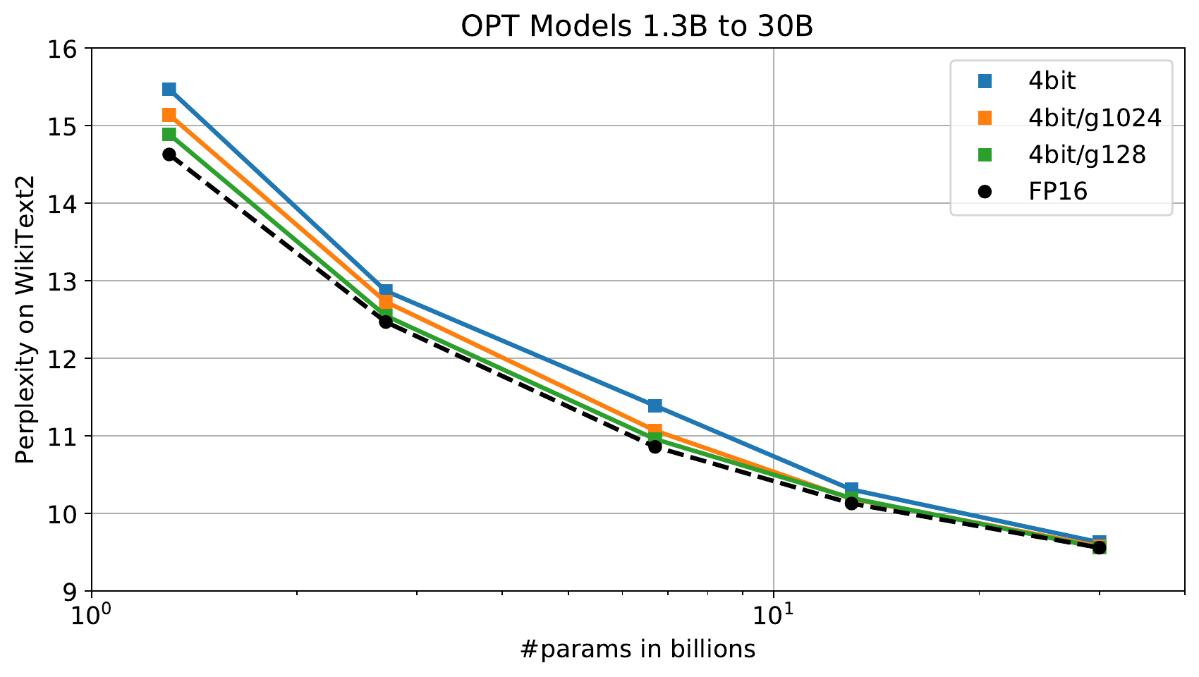
• Finer rulers per 128 columns (groupsize, gptq.py:120–128) are likewise in the code and an appendix, not the headline tables. Deployed GPTQ models essentially all use them.

I did not audit the CUDA kernel (quant_cuda_kernel.cu), so the speedup claims below rest on the paper alone.

Claims & evidence

One term first: perplexity is a standard score for language models on test text, where lower is better, and small differences matter; a jump from 8.3 to 110 means the model has stopped being a language model.

Claim	Evidence in paper	Verdict
4-bit OPT-175B is near-lossless: perplexity 8.34 → 8.37	Table in §5, consistent across OPT and BLOOM	verified — replicated widely since; 4-bit GPTQ became a default format
3-bit OPT-175B is usable (perplexity ≈ 8.68)	Same tables	partial — true for perplexity; later evaluations on question-answering tasks lose more than the perplexity delta suggests
175B quantized in ~4 GPU-hours on one A100	§5 runtime table	verified as reported, and consistent with the algorithm’s cost structure. I have not timed it myself.
3.25× (A100) / 4.5× (A6000) faster generation at 3-bit	Custom kernels, single-stream generation	unverified here — kernel not audited, and the numbers are for batch size 1, where memory reading dominates by construction
Accuracy loss negligible at all model sizes	Appendix tables	refuted as stated — the paper’s own small-model numbers degrade visibly. Bigger models quantize easier; the abstract just doesn’t dwell on it

Benchmarks

Perplexity on the WikiText2 test set, lower is better, from the paper:

Model	FP16 (original)	RTN 4-bit	GPTQ 4-bit	GPTQ 3-bit
OPT-175B	8.34	110.5	8.37	8.68
BLOOM-176B	8.11	8.37	8.21	8.64

Read the RTN column first; it carries the whole argument. Naive rounding turns OPT-175B into word salad (110.5) while GPTQ sits within noise of the original. Then read the BLOOM row and notice the argument wobble: BLOOM survives naive rounding almost intact, so how much the repair machinery buys depends on the model, for reasons nobody has fully pinned down.

Limitations & open questions

Weights only. The numbers flowing between layers (activations) stay 16-bit, so GPTQ says nothing about the harder regimes where those get quantized too; that thread runs through LLM.int8, SmoothQuant, and QuaRot.

Perplexity flatters quantization. A 0.03 change at 4 bits is probably safe. The 3-bit changes look small too, and then question-answering benchmarks lose real points. If a decision depends on it, evaluate the task you care about, not perplexity.

Two things I’d like answers to and don’t have: why 1% damping (the stabilizer added to $H$) is reliably enough, a magic constant every later repo inherits without analysis; and whether the clamping of drifted weights at the ruler’s edge costs anything measurable, since rulers are fitted before repairs start moving weights around.

Calibration sensitivity is under-explored. 128 chunks of English web text works for OPT and BLOOM; whether it works for a code model or a multilingual one is your problem to test.

Reproduction notes

Marked partial, and here is exactly what that means. On 2026-07-12 I read the reference implementation end to end at commit 2d65066 and matched it against the paper’s algorithm; that is the Paper-vs-code section. I also checked the mathematics numerically: the repair formula against a brute-force exact solve (agreement to fifteen decimals), and the correlated-two-inputs picture, the $\rho e$ absorption and the $(1-\rho^2)$ damage factor (holds to sampling noise). The script is published at verification/hessian-in-quantization/checks.py, and the sign-flip mistake I made on the first attempt is written up in the Hessian note. I have not re-run the quantization itself or re-measured any perplexity or speed number; every quantitative claim above is the paper’s.

The code audit changed my reading in one material way: the published method is fixed-order with one ruler per row, but the repo’s actorder and groupsize options are what the ecosystem standardized on, so “GPTQ” in a modern model card means something measurably better than “GPTQ” in the paper’s tables.

If you want to run it: opt.py still reads cleanly but predates several library API changes; the maintained path today is GPTQModel, the AutoGPTQ successor. Budget for the calibration-data download, not the math; the algorithm itself runs in minutes on small models.