The quantization white paper, five years later

Core insights. This is a tutorial, not a method paper, and its lasting contribution is a pair of recipes: a data-light PTQ pipeline (cross-layer equalization, then AdaRound, then careful range setting) that holds 8-bit models within 1% of float accuracy, and a QAT pipeline (fold the batch norms, initialize from the PTQ result, train through the rounding with a straight-through estimator) that makes 4-bit work. Nearly everything this site covers descends from vocabulary defined here. Reading it in 2026, three things stand out: the recipes aged well as structure even where the specific tricks died; the authors shipped the whole thing as a maintained toolkit (AIMET), which let me audit a white paper the way I’d audit a method repo; and one apologetic footnote about BERT (a few activations kept at 16 bits) is, in hindsight, the first published sighting of the outlier problem that LLM quantization has been fighting ever since.

Method

What simulated quantization actually simulates

The paper’s first service is defining the object of study. On real hardware, an int8 layer multiplies int8 weights against int8 activations into an int32 accumulator, adds int32 biases, and requantizes the result back to int8 for the next layer. Research code fakes this on GPUs with fake-quant nodes: quantize-then-dequantize operations inserted where the precision losses would occur, while everything still computes in floating point.

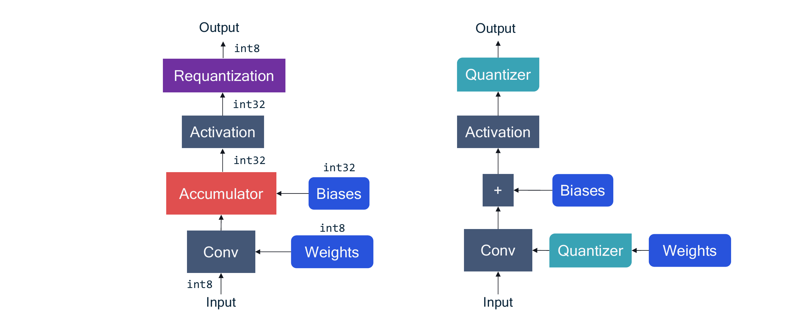
Two diagrams side by side. Left: on-device inference, where int8 weights and activations feed a Conv into an int32 accumulator with int32 biases, then activation and requantization back to int8. Right: the simulated version, where quantizer blocks wrap the weights and the layer output while computation stays in floating point. — **What the fake-quant graph stands in for.** Left, the actual integer pipeline with its int32 accumulator; right, the floating-point simulation with quantizer nodes at the places precision is really lost. Every QAT paper's forward pass is the right-hand picture; every deployment is the left one. Figure from the paper's LaTeX source — Nagel et al. (2021), arXiv:2106.08295

The grid itself is the same uniform affine quantizer we’ve now audited in three other notes: scale, zero point, integer clamp. The paper’s contribution is the decision table around it, defaults the field still uses: symmetric grids for weights (the zero-point multiplies against activations and would cost a data-dependent term otherwise), asymmetric for activations (post-ReLU distributions are one-sided; my check script measures a 4× MSE win for the zero point on rectified data), per-channel for weights where hardware allows. Every one of those defaults reappears verbatim in EfficientQAT’s quantizer and, with the symmetric-weights choice, in ParetoQ’s.

The PTQ recipe, and why each stage exists

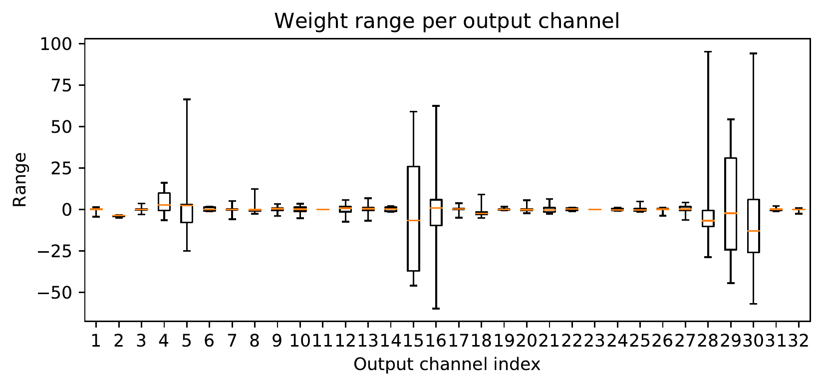
Flowchart of the standard PTQ pipeline: pre-trained FP model, then cross-layer equalization, then add quantizers with symmetric weights and asymmetric activations, then weight range setting by MSE, then a branch on data availability leading to AdaRound if calibration data exists or bias correction if not, then activation range setting. — **The standard PTQ pipeline.** Deliberately data-optional: the right branch exists specifically for the case where you have no calibration data at all. The 2021 field cared deeply about that constraint; the LLM era quietly abandoned it, since web text is always available. Figure from the paper's LaTeX source — Nagel et al. (2021), arXiv:2106.08295

Cross-layer equalization attacks a problem I hadn’t appreciated until seeing their MobileNetV2 plot: per-tensor weight quantization dies when one output channel’s range is 50× another’s, because the shared grid must span the widest channel. CLE fixes it without data, exploiting the positive homogeneity of ReLU: scale channel $i$ of one layer down by $s_i$ and the corresponding input column of the next layer up by $s_i$ , and the network function is exactly unchanged, while the ranges meet in the middle. The optimal scale is $s_i = \frac{1}{r_2^i}\sqrt{r_1^i r_2^i}$ , which equalizes the two layers’ per-channel ranges. I verified all three properties numerically: the formula matches AIMET’s implementation to machine precision, the ranges equalize exactly, and the function is preserved through ReLU to 1e-14.

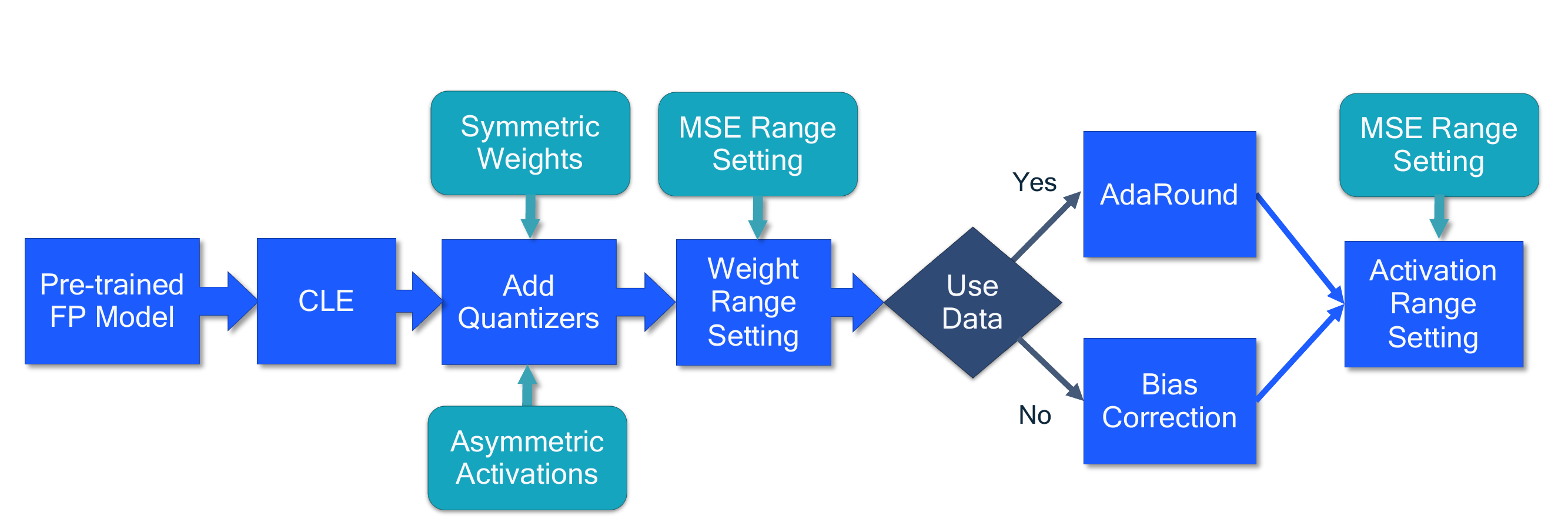
Box plot of weight ranges per output channel for a MobileNetV2 depthwise layer. Most of the 32 channels have ranges near zero, while a handful of channels span ranges of 50 to 100, dwarfing the rest. — **Why per-tensor quantization dies on MobileNetV2.** A few channels are 50–100× wider than the rest, so one shared grid wastes almost all its levels. This is the *weight-side* outlier problem; CLE solves this one. The activation-side version, which surfaced a year later in LLMs, has no such free fix. Figure from the paper's LaTeX source — Nagel et al. (2021), arXiv:2106.08295

AdaRound we’ve met in the Hessian note: round-to-nearest is provably suboptimal when weights interact, so learn the up/down choices per weight against a layer-wise reconstruction loss. The white paper presents the practical version: each weight gets a continuous variable $\alpha$ squashed through a rectified sigmoid (stretched by ζ=1.1, γ=−0.1 so it reaches exactly 0 and 1 at finite α, unlike a plain sigmoid), plus an annealed regularizer that starts permissive and ends by forcing every weight to commit to a corner. I verified both properties, and the constants in AIMET (defs.py:331–332) are the paper’s.

Range setting is the quiet workhorse: min–max ranges are one outlier away from disaster, so grid-search the clipping threshold minimizing quantization MSE. On a synthetic heavy-tailed tensor my check gets 2.9× lower error than min–max at 4 bits. It’s the same range-versus-resolution trade the ParetoQ note wrestles with around scale initialization, solved here by brute force in 2021.

The QAT recipe

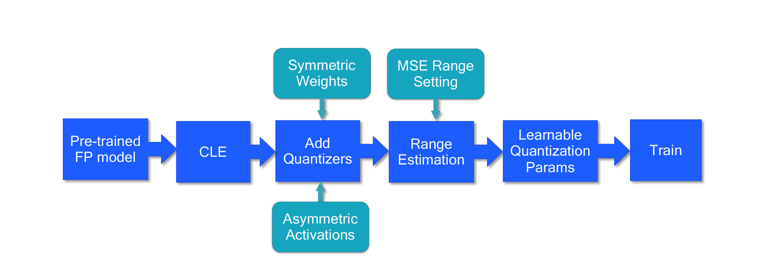
Flowchart of the standard QAT pipeline: pre-trained FP model, cross-layer equalization, add quantizers, range estimation, make quantization parameters learnable, then train. — **The standard QAT pipeline.** The important reading: QAT is initialized from the PTQ pipeline's output, not from scratch. "Do the cheap thing first and train from there" is the same architecture EfficientQAT rediscovered at block scale three years later. Figure from the paper's LaTeX source — Nagel et al. (2021), arXiv:2106.08295

The QAT chapter is where the STE, learnable ranges (LSQ-style), and batch-norm folding get their canonical treatment. Two of its practical findings shaped everything downstream. First, fold the batch norms before training and quantize the folded weights; training with unfolded BN then folding afterward re-breaks the quantization. Second, initialize QAT from a good PTQ state: their ablation shows range-learning QAT recovers from bad inits eventually, but starts points ahead from an MSE-calibrated one. Both findings transfer beyond CNNs; ParetoQ’s 90/10 budget split is the same “start from the best cheap state” instinct at a vastly larger scale.

Paper vs. code

The white paper’s companion implementation is AIMET (Qualcomm’s AI Model Efficiency Toolkit), built by the same group, and it makes this the rare tutorial you can audit line by line. Repo at commit 948a663, actively maintained in 2026.

What I could match directly:

Paper	Code
CLE scale $s_i = \frac{1}{r_2}\sqrt{r_1 r_2}$	`_aimet_common/cross_layer_equalization.py:492`, written as $r_1/\sqrt{r_1 r_2}$ ; algebraically identical (verified to 1e-16)
AdaRound rectified sigmoid, ζ=1.1, γ=−0.1	`_aimet_common/defs.py:331–332`; loss in `_base/adaround/adaround_loss.py` with the paper’s warm start and β annealing
MSE-based range setting	the encoding-analyzer grid search machinery
Uniform affine quantizer, symmetric weights / asymmetric activations defaults	throughout `quantsim`

What the code does that the paper doesn’t say:

CLE guards against degenerate channels: scale factors that come out NaN, infinite, or zero are silently reset to 1.0 (cross_layer_equalization.py:495–496). Dead channels strike again; every quantization implementation we’ve audited (GPTQ’s zeroed columns, this) carries an unstated epsilon-or-reset patch for inputs the math didn’t anticipate.
The 2026 AIMET has quietly become a museum of everything that came after the white paper: there’s a test_spinquant.py in the tree. The toolkit absorbed the rotation era its own paper predates.
And my favorite provenance find, in the LaTeX itself: a comment above the headline PTQ table admitting the numbers were assembled from multiple sources: “EfficientNet from the efficientnet slide deck, per-channel results from AdaRound slide deck.” The figures are literally exported corporate slides; one still has its “Confidential and Proprietary” footer in the PDF. Harmless, but a reminder that even the field’s textbook table is a collage, not one experiment.

Claims & evidence

Claim	Evidence in paper	Verdict
The PTQ pipeline holds W8A8 within ~1% of FP32 across CNNs and BERT	Table 10, eight models, averaged over 5 runs	verified as reported; consistent with half a decade of deployment practice since
W4A8 is achievable with PTQ (AdaRound)	Same table; e.g. ResNet-50 75.15 vs 76.07 FP	verified as reported, with one honest catastrophic exception they print: EfficientDet-D1 collapses to 0.31 per-tensor
QAT buys roughly one bit over PTQ	Table 11: W4A4 QAT ≈ W4A8 PTQ territory	partial; holds in their tables for CNNs, and the LLM era complicated it (see ParetoQ’s compensation/reconstruction boundary)
CLE + bias absorption makes MobileNetV2 W8A8 usable without data	CLE ablation: 0.1% → ~70% top-1	verified as reported; mechanism verified numerically here
BERT-base quantizes to W8A8 within 1%	Table 10, with the footnote: “a few quantized activations kept in 16 bits”	partial — true only with the escape hatch, and that footnote is the LLM outlier problem, eighteen months before LLM.int8 named it

Benchmarks

The headline PTQ table, condensed (top-1 / task metric, higher better, average of 5 runs):

Model	FP32	W8A8 (per-tensor)	W4A8 (per-channel)
ResNet-50	76.07	75.87	75.43
MobileNetV2	71.72	70.99	69.79
EfficientNet-lite	75.42	75.25	74.01
EfficientDet-D1	40.08	38.29	35.08
BERT-base (GLUE)	83.06	82.43	82.02

Read it with 2026 eyes and two things jump out. The 8-bit column was essentially a solved problem in 2021 for CNNs, which is why the interesting frontier moved to 4 bits and below. And the one transformer in the table needed special treatment (activations at 16 bits) that none of the CNNs did — the shape of the next five years of quantization research, visible in a single footnote if anyone had known to look.

Limitations & open questions

Time is the main one, and it cuts in specific, instructive ways. CLE’s exactness depends on positive homogeneity, which ReLU has and GELU/SiLU do not, so the white paper’s flagship data-free trick is mathematically inapplicable to every modern LLM; its spiritual successor is the rotation family (SmoothQuant’s scaling, QuaRot/SpinQuant), which trades exact invariance through nonlinearities for invariance around them. The per-channel-ranges problem CLE solved got solved differently at scale (per-group quantization, as in EfficientQAT’s g64). And the paper’s activation quantization assumes distributions a calibration set can capture, which emergent LLM outliers broke; the BERT footnote was the warning.

What survived untouched is the skeleton: the quantizer decision table, MSE range setting, STE-based QAT with learnable ranges initialized from PTQ, and the debugging mindset of its diagnostic flowchart. Reading ParetoQ’s recipe against this paper’s QAT chapter, the differences are scale and grid shape, not kind.

One methodological note: as a white paper, it reports no error bars beyond run averaging, compares against no external baselines, and (per the LaTeX comment) assembles numbers from internal decks. It’s a codified best-practices document from one excellent industrial lab, and should be read as exactly that, which is also why auditing it against their own toolkit, rather than against rival papers, is the right check.

Reproduction notes

Marked partial, meaning: on 2026-07-13 I read the white paper against AIMET at commit 948a663, matching the CLE mathematics, the AdaRound loss and its constants, and the quantizer defaults; that’s the Paper-vs-code section. I verified the core algorithms in NumPy: the CLE formula equivalence, exact range equalization, and function preservation through ReLU; the rectified sigmoid’s saturation and the annealed regularizer’s minima; MSE-vs-min-max range setting under outliers; and the asymmetric grid’s advantage on skewed data. The script is verification/quantization-whitepaper/checks.py, eight checks, all PASS.

What I did not do: rerun any of the model tables (the 2021 training setups are only sketched, and the LaTeX comment about slide-deck provenance suggests exact reproduction was never really on offer), or run AIMET end to end on a real network, which would be the natural next step if a question about the pipeline’s current behavior ever matters to a note.