SpinQuant, when rotations are worth learning

Method

Four rotation sites, two of them free

SpinQuant’s architecture map is the cleanest statement yet of where rotations can live in a transformer:

• R1, one hidden-size rotation threaded through the entire residual stream: folded into the embedding matrix and into every projection that reads from or writes to the stream. Mergeable, zero runtime cost.
• R2, one head-dimension rotation per layer between the V and O projections. Also mergeable, zero runtime cost.
• R3, a fixed Hadamard applied to queries and keys after RoPE, existing only to make the KV cache quantizable. Online, small runtime cost.
• R4, a fixed Hadamard on the down-projection’s input, taming the notorious SwiGLU activation outliers. Half folded into weights, half online.

R1 and R2 commute with everything on their paths, so they are exact symmetries of the full-precision network; R3 and R4 sit at spots (after RoPE, after the elementwise SwiGLU product) where no fold-through exists, which is why they stay fixed Hadamards rather than learned matrices. The learned/fixed split is the paper’s design insight: learn exactly the rotations that are free at inference, and only those.

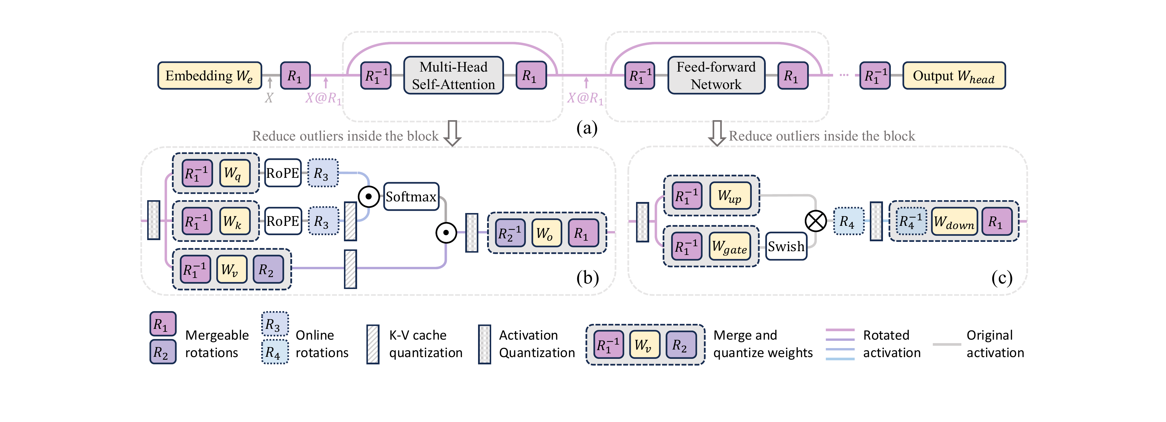
The invariance that makes R1 legal is worth spelling out, because it’s the same one the whole rotation era rests on: RMSNorm divides by the vector’s norm, and rotations preserve norms, so RMSNorm(Rᵀh) = Rᵀ·RMSNorm(h) exactly (after the norm’s scale vector γ is first folded into the adjacent weights, which is what fuse_norm_utils.py does before anything else). I verified both the commutation and the end-to-end fold-through numerically to 1e-15. This is also precisely the property that replaced the white paper’s CLE trick once GELU-era activations broke positive homogeneity: the 2021 pipeline’s data-free rescaling died with ReLU, and norm-rotation invariance is its successor.

Why learned: the lottery measurement

The paper’s Figure 1 is the whole motivation and deserves to be the famous one:

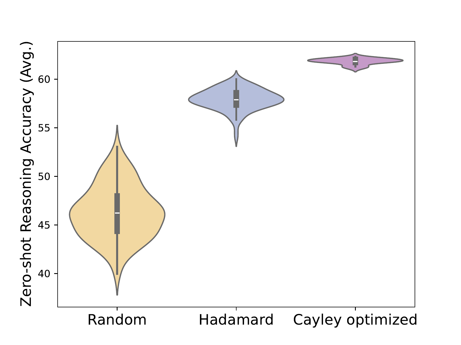
QuIP’s theory guarantees rotations land μ near the Gaussian floor with high probability, and that’s a statement about the bulk of rotations, not the best one. SpinQuant’s bet is that the tail of that distribution is reachable by gradient descent. My miniature check agrees: on a synthetic matrix with one structurally loud column, a Cayley-parameterized rotation optimized by finite-difference descent beats the best of twenty random rotations by a further 30% in 4-bit quantization error.

The math, slowly

Three small objects underneath all the notation. First, the norm trick that makes R1 free: RMSNorm only measures a vector’s length, and rotations preserve lengths. Take $h = (3, 4)$, length 5; rotate by 90° to $(-4, 3)$, length still 5, so $\mathrm{RMSNorm}(Rh) = Rh/5 = R\cdot\mathrm{RMSNorm}(h)$. The rotation slides through the normalization, which is why the whole residual stream can be rotated with the function unchanged while every quantizer sees different, tamer numbers.

Second, the direction of change of a rotation is a skew-symmetric matrix ($A^\top = -A$). In 2D every skew matrix is $\begin{bmatrix} 0 & -t \\ t & 0\end{bmatrix}$, the infinitesimal “rotate counterclockwise at speed $t$.” Skew matrices are the velocities of rotations, and they’re what gradients get projected onto.

Third, the Cayley transform turns a velocity into an exact rotation: $Q = (I - A)(I + A)^{-1}$. Orthogonality is a two-line proof: skewness gives $(I-A)^\top = I+A$, and $(I\pm A)$ commute (both are polynomials in $A$), so everything in $Q^\top Q$ cancels to $I$. A case you can do by hand: $t=1$ gives $(I-A) = \begin{bmatrix}1&1\\-1&1\end{bmatrix}$, $(I+A)^{-1} = \tfrac12\begin{bmatrix}1&1\\-1&1\end{bmatrix}$, and their product is exactly $\begin{bmatrix}0&1\\-1&0\end{bmatrix}$, a perfect 90° rotation (in general, 2D Cayley of speed $t$ rotates by $2\arctan t$). This example is in my check script, exact to the last bit.

Gradient descent over rotations is then a three-step dance, and the phrase to keep is you never add to a rotation, you rotate it a little, in the best direction:

1. backprop an ordinary, constraint-ignorant gradient $G = \partial L/\partial R$;
2. project it to a velocity: $W = GR^\top - RG^\top$, automatically skew, keeping exactly the part of $G$ that a rotation can act on;
3. retract: $R \leftarrow (I - \tfrac t2 W)^{-1}(I + \tfrac t2 W)\,R$, exactly orthogonal at any step size.

Cayley SGD, or how to descend without leaving the manifold

The optimization problem is: minimize the quantized network’s cross-entropy over orthogonal matrices R1, R2, with all weights frozen. Plain gradient steps would immediately break orthogonality, so the repo uses Cayley SGD (train_utils/optimizer.py, adapted with credit from Li et al.’s Stiefel-manifold code): project the gradient to a skew-symmetric tangent, then move along the Cayley retraction, which maps skew matrices to orthogonal ones. My checks verify the parameterization exactly (a Cayley transform of any skew matrix is orthogonal to machine precision) and document a real property of the implementation: the optimizer approximates the retraction with a short fixed-point loop, so training iterates are only approximately orthogonal, converging at roughly 1000× error reduction per doubling of loop iterations.

The recipe, from the paper’s appendix and the repo’s scripts, is strikingly light: 100 steps, learning rate 1.5, batch size 1, 800 WikiText-2 samples (their ablation shows 128 samples suffices), bf16, quantizers active in the forward pass with straight-through gradients. That’s 30 minutes for Llama-3-8B, versus 20 minutes for the GPTQ pass that follows. The learning rate of 1.5 stops looking exotic once you note the parameters live on a bounded manifold; there is no runaway direction to fear. After training, R1 and R2 are folded into the checkpoint, and standard PTQ (RTN or GPTQ) quantizes the rotated model.

Note what the loss is, because it places this method precisely among the site’s other notes: the actual end-to-end cross-entropy of the quantized network, not a per-layer proxy, optimized over a parameter set of roughly 17M (one 4096² R1 plus 32 head-size R2’s, about 0.2% of an 8B model). That tiny, manifold-constrained hypothesis class is also the honest answer to why 100 steps and a few hundred samples don’t overfit. The collection now forms a ladder of “which objective, over which parameters”:

Method	Objective	Trainable
GPTQ / QuIP	per-layer proxy $\mathrm{tr}(EHE^\top)$	nothing (closed form)
SpinQuant	end-to-end cross-entropy	rotations, ~0.2%
EfficientQAT E2E-QP	end-to-end cross-entropy	scales, ~1.6%
ParetoQ	end-to-end cross-entropy	everything

Each step down the ladder buys accuracy with compute; SpinQuant’s row is the cheapest entry into end-to-end territory that exists.

Paper vs. code

Repo: facebookresearch/SpinQuant at commit 8f47aa3, official. optimize_rotation.py (rotation training), eval_utils/rotation_utils.py (the folds), train_utils/apply_r3_r4.py (online rotations), train_utils/optimizer.py (Cayley SGD).

What I could match directly:

Paper	Code
Trainables are exactly R1 + per-layer R2	optimize_rotation.py: the optimizer receives [model.R1.weight] plus each layer’s R2.weight, nothing else
R1 folded into embeddings, all stream-facing projections, head	rotation_utils.py:55–111
R2 folded into v_proj/o_proj per head	rotation_utils.py:114–119
R3 on Q,K after RoPE for KV quantization	QKRotationWrapper, apply_r3_r4.py:37, monkeypatched over the RoPE function
R4 half-folded into down_proj, half online	apply_r3_r4.py:14–19
Cayley SGD on the Stiefel manifold	SGDG, optimizer.py:57, credited to Li et al.’s reference implementation
100 iterations, lr 1.5, 800 samples	scripts/10_optimize_rotation.sh

What the code does that the paper doesn’t say:

• Tied embeddings break the method. For Llama-3.2-style models with tie_word_embeddings, R1 folds differently into the embedding (right-multiply) and the head (left-multiply by the transpose), so the code silently unties them by cloning lm_head from embed_tokens (optimize_rotation.py:47–50, comment included). A real constraint on the approach that only exists in a code comment.
• K-cache quantization requires power-of-2 head dims (apply_r3_r4.py:44, an assert), since R3 relies on the fast Hadamard transform. True for Llama, an obstacle elsewhere.
• The fixed-point Cayley loop means training-time rotations drift slightly off the manifold between steps, as quantified in my checks; harmless at these step counts, unstated anywhere.
• The repo is also a deployment artifact: an ExecuTorch export path (31_optimize_rotation_executorch.sh, group-size 256/32 4-bit weights with 8-bit dynamic activations), which is the pipeline behind Meta’s officially released quantized Llama-3.2 models (the HuggingFace checkpoints literally named Llama-3.2-1B-Instruct-SpinQuant_INT4). Of everything covered on this site, this is the method most concretely running on consumer devices.

Claims & evidence

Zero-shot average below = eight commonsense tasks; W-A-KV notation gives weight, activation, and KV-cache bits.

Claim	Evidence in paper	Verdict
Rotation quality is a lottery worth optimizing	Fig. 1 violin: ~13-point spread across random rotations at 4-bit	verified as reported, and reproduced in miniature in my checks (learned beats best-of-20 random by 30%)
Learned rotations beat QuaRot’s random Hadamards	Head-to-head table: Llama-3-8B W4A4KV4, 65.5 vs 63.3 with GPTQ; Llama-3-70B, 69.3 vs 65.1	verified as reported; QuaRot is concurrent work re-run by these authors, with the usual caveat that implies
Random rotations can catastrophically fail at scale	Llama-3-70B W4A4KV4 with RTN: QuaRot 41.3 avg / 92.4 ppl vs SpinQuant 70.1 / 4.1	verified as reported, the single most dramatic number in the paper
W4A4KV4 Llama-3-8B lands ~4 points from FP	Detail table: 65.5 avg vs 69.6 FP, ppl 7.3 vs 6.1	verified as reported
100 iterations and few samples suffice	Appendix ablation: stable from 128 samples, plateau at 100 iterations	verified as reported; consistent with only ~30M trainable rotation parameters
Rotations preserve the FP network exactly	Invariance argument, Sec. 3	verified numerically here (RMSNorm commutation and fold-through to 1e-15), for R1/R2; R3/R4 are exact by construction but add runtime ops

Benchmarks

The decisive comparison, Llama-3 models at W4A4 (their Table 6; FP baselines 69.6 and 74.5):

Method	8B, KV16	8B, KV4	70B, KV16	70B, KV4
QuaRot + RTN	59.5	58.6	41.5	41.3
SpinQuant + RTN	64.6	64.1	70.1	70.1
QuaRot + GPTQ	63.8	63.3	65.4	65.1
SpinQuant + GPTQ	65.8	65.5	69.5	69.3

Two readings. At 8B the learned rotations are worth ~2 points over random Hadamards, a solid but ordinary margin. At 70B the gap becomes qualitative: with plain RTN rounding, QuaRot’s configuration collapses outright (perplexity 92) while SpinQuant with no GPTQ at all sits within 4.4 points of full precision. Learned rotations don’t just polish the average case, they remove the tail risk that grows with model size. The GPTQ-vs-RTN spread inside SpinQuant’s own rows is also worth noticing: after good rotations, GPTQ is worth less than a point at 70B, an echo of QuIP’s finding that once the distribution is fixed, the rounding barely matters.

Limitations & open questions

The rotations are per-model artifacts. Every new checkpoint needs its own 100-step optimization, and the learned matrices are meaningless for any other model; random Hadamards are universal. Thirty minutes is cheap, but it’s a pipeline stage QuaRot doesn’t have.

The comparison surface is friendly. QuaRot numbers are these authors’ re-runs; the two papers are concurrent, use different clipping and calibration choices, and later work (OSTQuant, FlatQuant) claims further gains over both with learnable scaling and affine transforms respectively. I have not audited those.

W4A4 activation quantization remains the hard regime the site’s other notes mostly avoid, and the absolute gaps here (4+ points at 8B) are far from free. Weight-only readers should note SpinQuant’s weight-only results exist but the paper’s center of mass, and its deployment story, is W4A8-ish on-device inference.

And the open question this note inherits from three others: rotations composed with real QAT. The first authors of this paper went on to write ParetoQ without rotations; the rotate-then-train experiment sits untouched between their own two papers.

Reproduction notes

Marked partial, meaning: on 2026-07-14 I read the rotation training entry point, the fold utilities, the R3/R4 application, and the Cayley optimizer end to end at commit 8f47aa3 and matched them against the paper; that’s the Paper-vs-code section. I verified the mathematical spine numerically: Cayley transforms of skew matrices are exactly orthogonal; the 2D Cayley transform at unit speed is exactly a 90-degree rotation; the exact Cayley retraction preserves orthogonality while the code’s fixed-point approximation converges to it (~1000× per iteration doubling); RMSNorm commutes with rotations and the folded norm-linear path is exactly invariant; and a Cayley-optimized rotation beats the best of twenty random rotations on a structured-outlier matrix. The script is verification/spinquant/checks.py, seven checks, all PASS.

What I did not do: run rotation optimization on a real model (30 GPU-minutes for an 8B, the second-cheapest true reproduction available across these notes, after nothing), or evaluate Meta’s released SpinQuant Llama-3.2 checkpoints against the paper’s tables, which would close the loop on the deployment claim.