QuIP, the theorem behind the rotation trick

Method

The proxy loss, one more time

QuIP starts from the same layer-wise objective as the GPTQ note and the Hessian note: minimize $\mathrm{tr}\big((W - \hat W)H(W - \hat W)^\top\big)$ with $H$ the second-moment matrix of the layer’s inputs. Nothing new yet, and that’s deliberate; the paper’s contribution is to treat this object with actual theory rather than heuristics.

LDLQ, and the theorem that closes the rounding question

Write $H = L D L^\top$ with $L$ unit lower triangular (the LDL decomposition, a cousin of Cholesky). QuIP’s rounding algorithm, LDLQ, quantizes one column at a time with a linear feedback correction: each column is rounded after adding a combination, given by the corresponding column of $L$, of the errors already committed on previously-quantized columns. In the audited code this is nine lines (vector_balance.py:171–180): factor, normalize, loop backward, round with feedback.

The math, slowly

Before the theorems, the machinery, because it’s simpler than the notation suggests. Any symmetric positive-definite $H$ factors as $H = LDL^\top$ with $L$ unit lower triangular (ones on its diagonal) and $D$ diagonal. A 2×2 you can check by hand:

$$H = \begin{bmatrix} 1 & 0.8 \\ 0.8 & 1 \end{bmatrix} = \begin{bmatrix} 1 & 0 \\ 0.8 & 1 \end{bmatrix} \begin{bmatrix} 1 & 0 \\ 0 & 0.36 \end{bmatrix} \begin{bmatrix} 1 & 0.8 \\ 0 & 1 \end{bmatrix}.$$

Read $D$ as leftover variance: $D_{22} = 1 - 0.8^2$ is what remains of direction 2 after direction 1 explains what it can. Strong correlations mean small $D$ entries, and $\mathrm{tr}(D) = 1.36$ here against $\mathrm{tr}(H) = 2$.

Now run the algorithm on one weight row $w = [0.4,\ 0.3]$, rounding to integers. Column 2 goes first (the loop runs backward) with no feedback: $\hat w_2 = \mathrm{round}(0.3) = 0$, committing error $0.3$. Column 1 then receives feedback $(w_2 - \hat w_2)\cdot L_{21} = 0.3 \times 0.8 = 0.24$, and rounds $0.4 + 0.24 = 0.64$ to $\hat w_1 = 1$. Notice it rounded $0.4$ up to 1, deliberately away from its nearest integer, because the correlation says this error will cancel against the one already committed. Compare: nearest rounding $\hat w = [0,0]$ has proxy loss $0.442$; LDLQ’s $[1, 0]$ has $0.162$, a 2.7× win purchased by rounding one weight the “wrong” way. This is the same compensation instinct as GPTQ, expressed as a single linear filter instead of a loop of Hessian updates.

Why $\mathrm{tr}(D)$ appears in the theorems is one identity. Let $\eta_i = \hat w_i - (w_i + \text{feedback}_i)$ be the per-step round-off, always in $[-\tfrac12, \tfrac12]$. The factorization makes the total error $E = \eta L^{-1}$, and then

$$\mathrm{tr}(E H E^\top) = \mathrm{tr}\big(\eta L^{-1} \cdot LDL^\top \cdot L^{-\top} \eta^\top\big) = \mathrm{tr}(\eta D \eta^\top).$$

The $L$‘s cancel exactly: LDL feedback is precisely the choice that makes the coupled metric $H$ act like the diagonal $D$ on your rounding noise. In the worked example, $\eta = [0.36, -0.3]$ and $1.0(0.36)^2 + 0.36(0.3)^2 = 0.162$, matching the loss computed the long way. My check script verifies this identity to machine precision on random instances. Once cross-terms are gone, each noise entry contributes $D_{jj}\eta_j^2$ independently, and $|\eta|\le\tfrac12$ gives the $\frac m4\mathrm{tr}(D)$ worst case and $\frac m{12}\mathrm{tr}(D)$ average immediately. Optimality within the class follows from the same picture: any other feedback leaves coupling behind, and coupling only adds.

Two theorems make this more than another rounding heuristic. First, within-class optimality: among all rounding schemes whose feedback matrix depends on $H$ alone, LDLQ achieves the minimum worst-case and average-case proxy loss, exactly $\frac{m}{4}\mathrm{tr}(D)$ and $\frac{m}{c}\mathrm{tr}(D)$ with $c = 12$ for nearest rounding. I verified the average-case formula by Monte Carlo: over 4,000 random weight matrices, the empirical proxy loss matches $\frac{m}{12}\mathrm{tr}(D)$ to within 0.3%. Second, GPTQ is in the class: the paper proves OPTQ (GPTQ’s publication name) is exactly equivalent to LDLQ, which means the workhorse algorithm the community adopted for engineering reasons was, unknowingly, already the optimal member of its family. The repo ships its own equivalence checker (optq_ldlq_equiv.py), which I appreciate as a house-style kindred spirit; my independent NumPy check reproduces the equivalence to exact equality, zero difference across all entries, once both are run on the integer lattice with matching rounding conventions.

The strategic consequence deserves emphasis because it explains the next three years of the field. If the rounding step is provably optimal given $H$, no cleverer rounding can rescue 2-bit quantization. The only remaining lever is the conditioning of the problem itself: change $W$ and $H$ into equivalent matrices that round better.

Incoherence, and the rotation that manufactures it

QuIP defines the lever precisely. A Hessian is μ-incoherent if no eigenvector entry exceeds $\mu/\sqrt{n}$; a weight matrix if no entry exceeds $\mu\lVert W\rVert_F/\sqrt{mn}$. In words, for weights: μ is how many times larger than the root-mean-square entry the worst entry is. Numbers make it concrete: a 4096×4096 Gaussian matrix has $\mu \approx \sqrt{2\ln(mn)} \approx 5.8$ (the expected extreme of that many samples), while a single outlier at 50× the RMS makes $\mu = 50$ regardless of everything else. Small μ means no outliers and no aligned structure, exactly the regime where a uniform grid wastes nothing. The theory then bounds LDLQ’s loss by $\frac{m\mu^2}{4n}\,\mathrm{tr}(H^{1/2})^2$, so incoherence plus the (empirically strong) low-rank structure of real Hessians yields an asymptotic factor-of-$\mu^2 k/n$ advantage over plain rounding. There’s also a converse the successors rarely cite: without the incoherence assumption, no spectral bound can separate LDLQ from stochastic rounding at all. The assumption isn’t decoration; it’s load-bearing.

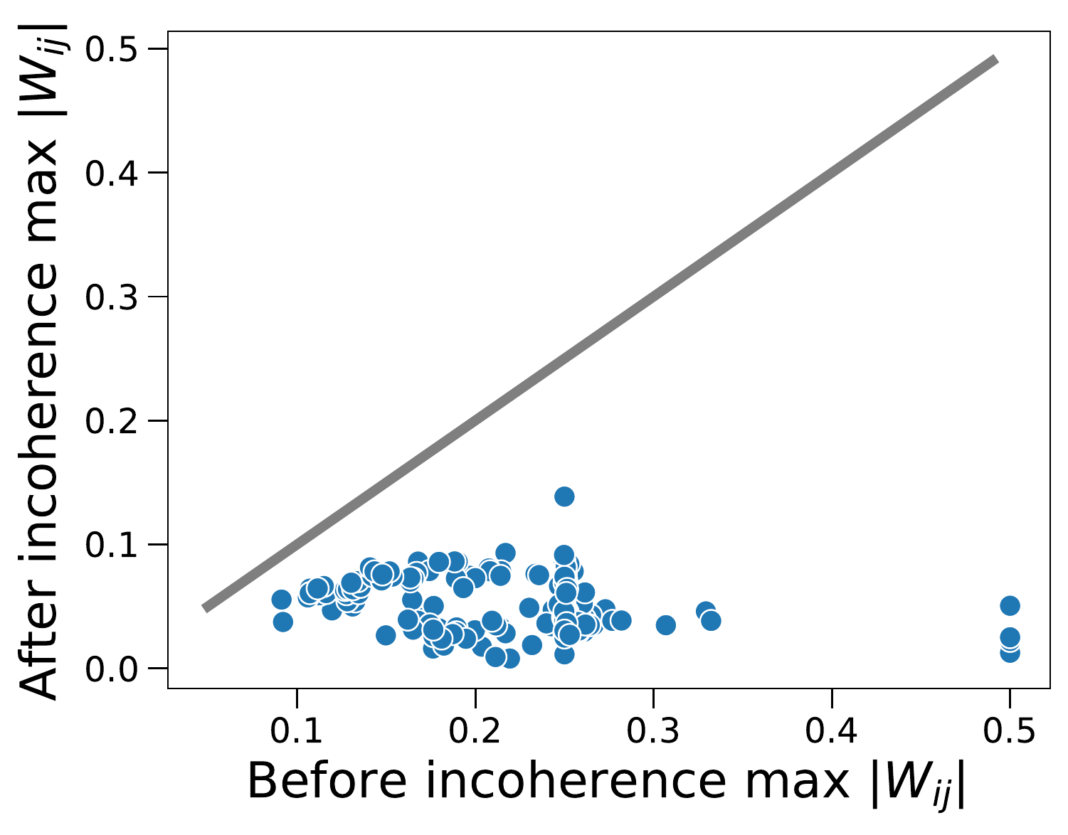
Manufacturing incoherence is the famous part. Draw random orthogonal matrices $U, V$ and transform $W \mapsto UWV^\top$, $H \mapsto VHV^\top$. The proxy loss is exactly invariant (a two-line trace identity, verified numerically in my checks), the network can absorb the rotations at its boundaries, and with high probability both matrices land at μ near the Gaussian floor $\sqrt{2\log(mn)}$. My check plants 25σ outliers in a 64×64 matrix and watches a random rotation take μ from 13.2 to 4.4, which is the Gaussian level for that size; rotation cannot do better than “make it Gaussian,” and doesn’t need to. For efficiency, QuIP builds $U, V$ as Kronecker products of small random orthogonals shuffled by permutations (the “butterfly” construction, method.py:16–77), trading a dense matrix multiply for a few small ones. Its successors replaced this with the randomized Hadamard transform, but the job description was written here.

And the question I always end up asking of these methods: what actually runs at inference? QuIP stores the rotated quantized weights $\tilde W = UWV^\top$, so each linear layer computes $y = U^\top(\tilde W\,(Vx))$: rotate the incoming activations by $V$, multiply by the cheap 2-bit matrix, rotate the result back by $U^\top$. The butterfly structure keeps those two extra multiplies from costing a full dense matmul each, and since $U, V$ are pseudorandom you store seeds, not matrices. The runtime tax is real, though, and this repo makes no serious attempt at fast kernels; folding the rotations into neighboring layers so they cost nothing (QuaRot) and building tensor-core Hadamard kernels (HadaCore) is exactly the engineering the successors contributed.

One more code-level observation that I haven’t seen credited: after rotating, QuIP quantizes on a symmetric grid with no zero level, scaled by the Frobenius norm rather than min–max (quant.py:10–15: four levels at $\{-1, -\tfrac{1}{3}, +\tfrac{1}{3}, +1\}\cdot s$ for 2 bits). That is the same zero-free symmetric family that ParetoQ’s SEQ arrives at two years later for 2-bit QAT, motivated by the same logic: rotated (or retrained) weights are dense and zero-centered, so spending a level on exact zero is a waste. The ParetoQ note treats that grid as a discovery of the QAT era; the shape was sitting in QuIP’s quant.py all along.

Paper vs. code

Repo: Cornell-RelaxML/QuIP at commit ac92cfc, official. Compact and readable: method.py (232 lines, preprocessing), vector_balance.py (rounding), quant.py (grids).

What I could match directly:

Paper	Code
LDLQ with linear feedback from the LDL factors	vector_balance.py:171–180; my reimplementation matches GPTQ-style compensation exactly
Two-sided incoherence transform, proxy-invariant	method.py:157–180 (forward), 195–205 (undo)
Kronecker/butterfly random orthogonals	method.py:16–77, four variants selectable
Frobenius-scaled symmetric grid after rotation	quant.py:10–15 (qfnb)
GPTQ compatibility path (dead columns, damping)	preproc_gptqH, method.py:182–192, lifted from the GPTQ codebase

What the code does that the paper’s method section doesn’t say:

• There’s a diagonal rescaling stage before the rotation: weights and Hessian are rebalanced by $\sqrt[4]{\mathrm{diag}(H)/\mathrm{diag}(W^\top W)}$ per column (method.py:139–154). A SmoothQuant-style equalization quietly runs inside “incoherence processing”; the ablation flags exist (preproc_rescale), but a reader of the method section alone would not know the shipped pipeline does this.
• The Hessian gets a trace-normalized ridge: $H \leftarrow H\cdot n/\mathrm{tr}(H) + 0.01 I$ (method.py:173). That’s a substantial fixed damping on top of the optional GPTQ-style 1% — the same magic-constant genre we flagged in every other note, here with an extra normalization nobody mentions.
• The butterfly construction has four variants (blocking, permutation on/off, dense), with the default differing from the paper’s description (variant 1, “no blocking”).
• llama.py exists: Llama support was added post-publication, but the paper’s tables are OPT-only, and the README points Llama users to QuIP# instead.

Claims & evidence

Claim	Evidence in paper	Verdict
First 2-bit LLM quantization with usable quality	OPT-30B: Wiki 11.48 vs FP 9.56, vs GPTQ’s 71.7 (Table, baseline block)	verified as reported for OPT-scale models; “usable” is doing work, see Benchmarks
GPTQ ≡ LDLQ (within-class optimal)	Theorem + proof, Sec. 4; repo ships an equivalence script	verified — my independent implementation reproduces exact equality
$L_{avg} = \frac{m}{12}\mathrm{tr}(D)$ for LDLQ-nearest	Theorem (thmLDLopt)	verified by Monte Carlo to 0.3%
Random orthogonal transforms yield μ-incoherence w.h.p.	Concentration lemmas, Sec. 3	verified empirically (μ 13.2 → 4.4, at the Gaussian floor); the probabilistic bound itself I read but did not re-derive
Incoherence is necessary for the spectral advantage	No-improvement theorem (thmOPTQequivNearStoch)	unverified here — proof read, not checked
Guarantees for the full quantized network	Bounds are for the per-layer proxy loss only	partial — the title says “with guarantees”; the guarantees stop at the proxy, and the paper is upfront about this in the body

Benchmarks

OPT-30B, from the paper’s own table, the cleanest before/after in the quantization literature:

Rounding	Processing	W4 Wiki ppl	W3	W2
FP16	n/a	9.56	9.56	9.56
GPTQ/LDLQ	baseline	9.59	10.32	71.70
Nearest	baseline	10.77	1,565	41,548
GPTQ/LDLQ	incoherence	9.60	9.79	11.48
Nearest	incoherence	9.77	9.89	12.04

Read the columns right to left. At 4 bits, processing barely matters and even nearest rounding works: the problem is easy. At 2 bits, the baseline column is a graveyard at any rounding sophistication, and incoherence processing rescues both algorithms, compressing the gap between clever LDLQ and dumb nearest from three orders of magnitude to five percent. That last observation is the theory made visible: once the distribution is incoherent, the rounding barely matters, exactly as the optimality theorem says it shouldn’t.

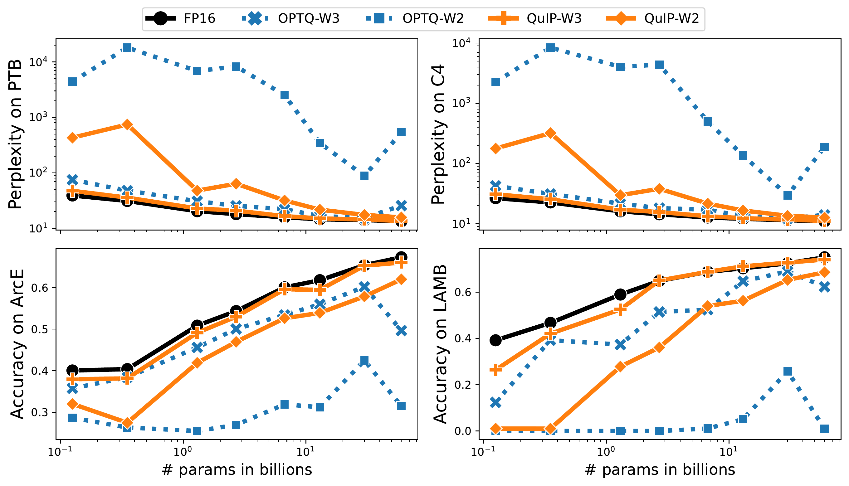
Honesty about the absolute numbers: 11.48 against 9.56 is a real gap, “usable” not “lossless,” and it’s on OPT, a family that later work showed is unusually quantization-friendly at the top end. The Llama-era numbers that made 2-bit genuinely competitive belong to the successors (QuIP#‘s lattice codebooks, QTIP’s trellises, plus fine-tuning), all built on this paper’s two rails.

Limitations & open questions

The guarantees are proxy-loss guarantees. Nothing bounds end-task degradation, and the gap between “layer outputs preserved” and “model behavior preserved” is exactly the compensation-regime blindness discussed in the Hessian note. The title oversells by one word; the body doesn’t.

Everything is OPT, evaluated pre-Llama, weights-only, and without fine-tuning. Each of those gaps became someone’s paper: rotations for activations (QuaRot), learned rotations (SpinQuant), codebooks plus fine-tuning on the incoherent representation (QuIP#, QTIP).

The rotations cost inference compute: the butterfly matvecs must run at load or runtime, and this repo makes no serious attempt at fast kernels. The Hadamard-kernel infrastructure that makes rotation ~free came later (HadaCore and friends).

And a question the paper leaves open that I find genuinely interesting after our QAT notes: LDLQ’s optimality is within the class of fixed linear feedbacks computed from H. Training-based methods (AdaRound’s learned directions, full QAT) sit outside the class, which is precisely why they can still beat it. The theorem draws the boundary of what calibration-only methods can achieve; it does not fence in learning.

Reproduction notes

Marked partial, meaning: on 2026-07-13 I read method.py, vector_balance.py, and quant.py end to end at commit ac92cfc and matched them against the paper’s algorithms and theorem statements; that’s the Paper-vs-code section. I verified seven claims numerically in NumPy: the exact proxy-loss invariance of the incoherence transform; the μ collapse to the Gaussian floor under random rotation; the LDLQ–GPTQ equivalence, reproduced constructively to exact equality; the average-case optimality formula $\frac{m}{12}\mathrm{tr}(D)$ by Monte Carlo; the cancellation identity $\mathrm{tr}(EHE^\top) = \mathrm{tr}(\eta D \eta^\top)$ from the math section, exact on random instances; the $|\eta| \le \tfrac12$ noise bound; and a miniature of the 2-bit step function (2.5× proxy-loss improvement from rotation alone on an outlier-planted matrix). The script is verification/quip/checks.py, all PASS.

What I did not do: run the pipeline on an actual OPT model (the repo predates current transformers and the README itself redirects users to QuIP#), or re-derive the concentration lemmas and the necessity theorem, which I read and found plausible but only spot-checked empirically.